AD, AS and Related Concepts - Revision Notes
CBSE Class–12 economics
Revision Notes
Macro Economics 07
Determinations of Income and Employment
Aggregate Demand refers to total value of all final goods and services that are planned to buy by all the sectors of the economy at a given level of income during a period of time. AD represents the total expenditure on goods and services in an economy during a period of time.
Components of Aggregate demand are:
(i) Household consumption expenditure (C).
(ii) Investment expenditure (I).
(iii) Govt. consumption expenditure (G).
(iv) Net export (X – M).
Thus, AD = C + I + G + (X – M)
In two sector economy AD = C + I
Aggregate Supply is the money value of all final goods and services available for purchase by an economy during a given period. It is the flow of goods and services in the economy. Since, money value of final goods and services is equal to net value added, AS is nothing but the national income.
AS = C + S
Aggregate supply represents the national income of the country.
AS = Y (National Income)
Consumption function shows functional relationship between consumption and Income.
C = f(Y)
where C = Consumption
Y = Income
f= Functional relationship.
Equation of Consumption Function
C =  + MPC * Y
C = Consumption
= Autonomous consumption.
MPC(b)= Marginal Propensity to consume
does not changed/affected by change in income. It is minimum level of consumption , even when income is zero. Consumption expenditure at zero level of income is called autonomous consumption. It is income inelastic.
Induced consumption is the expenditure which is affected by change in income. It is indicated by MPC × Y. Induced consumption is the portion of consumption that varies with disposable income.
Propensity to consume:- It is a schedule that shows consumption expenditure at different levels of income in an economy.
Consumption function (propensity to consume) is of two types:
(a) Average propensity to consume (APC)
(b) Marginal propensity to consume (MPC)
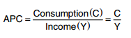
Average propensity to Consume (APC): It refers to the ratio between total consumption(C) and total income(Y) at given level of income in the economy.
Important Points about APC
(i) APC is more than 1: as long as consumption is more than national income before the break-even point, APC > 1.
(ii) APC = 1, at the break-even point, consumption is equal to national income.
(iii) APC is less than 1: beyond the break-even point. Consumption is less than national income.
(iv) APC falls with increase in income.
(v) APC can never be zero: because even at zero level of national income, there is autonomous consumption.
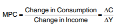
Marginal Propensity to Consume (MPC): Marginal propensity to consume refers to the ratio of change in consumption expenditure to change in income.
Important Points about MPC
(1) Value of MPC varies between O and 1: If the entire additional income is consumed, then ΔC = ΔY, making MPC = 1. However, if entire additional income is saved, than ΔC = 0, making MPC = 0
(2) MPC is the slope of consumption curve and remain constant throughout in the short run.
(3) Value of APC > MPC
Saving function refers to the functional relationship between saving and national income.
S = f (y)
Equation of Saving function
S =  +MPS.Y
where S = saving
Y = National Income
f = Functional relationship.
Saving function (Propensity to Save) is of two types.
(i) Average Propensity to Save (APS)
(ii) Marginal propensity to Save (MPS)
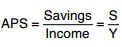
Average Propensity to Save (APS): Average propensity to save refers to the ratio of savings to the corresponding level of income
Important Point about APS
(1) APS can never be 1 or more than 1 :As saving can never be equal to or more than income.
(2) APS can be zero: At break even point C = Y, hence S = 0
(3) APS can be negative: At income levels which are lower than the break-even point, APS can be negative when consumption exceeds income.
(4) APS rises with increase in income.
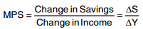
Marginal Propensity to Save (MPS): Marginal propensity to save refers to the ratio of change in savings to change in total income.
MPS varies between 0 and 1
(i) MPS = 1 if the entire additional income is saved. In such a case, ΔS = ΔY, then MPS = 1
(ii) MPS = 0 If the entire additional income is consumed. In such a case, ΔS = 0, then MPS = 0
(iii) Mps is the slope of saving curve.
(iv) MPS remains constant throughout in short run.
Relationship between APC and APS
The sum of APC and APS is equal to one. It can be proved as under we know:
APC + APS = 1
Y = C + S
Dividing both sides by Y, we get
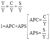
APC + APS = 1
because income is either used for consumption or for saving.
Relationship between MPC and MPS
The sum of MPC and MPS is equal to one. It can be proved as under:
MPC + MPS = 1
We know
ΔY = ΔC + ΔS
Dividing both sides by ΔY, we get
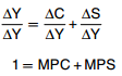
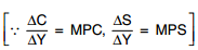
MPC + MPS = 1 because total increment in income is either used for consumption or for saving.
Investment refers to the expenditure incurred on creation of new capital assets.
The investment expenditure is classified under two heads:
(i) Induced investment
(ii) Autonomous investment.
Induced Investment: Induced investment refers to the investment which depends on the profit expectations and is directly influenced by income level (only for reference).
Autonomous Investment: Autonomous investment refers to the investment which is not affected by changes in the Level of income and is not induced solely by profit motive. It is income inelastic.
Ex-Ante Savings: Ex-ante saving refers to amount of savings which all the household intended to save at different levels of income in the economy at the beginning of period. It is also known as planned savings.
Ex-Ante Investment: Ex-ante investments refers to amount of investment which all the firms plan to invest at different level of income in the economy at the beginning of the period. It is also known as planned investment.
Ex-Post Saving: Ex-post savings refer to the actual or realised savings in an economy during a financial year at end of the period.
Ex-Post Investment: Ex-post investment refers to the actual or realised investment in an economy during a financial year at the end of the period.
Equilibrium level of income is determined only at the point where AD = AS or S = I, .i.e. the flow of goods and services in the economy is equal to the demand for goods and services But it cannot always be at full employment level also as it can be at less than full employment.
Full employment is a situation when all those who are able and willing to work at prevailing wage rate, get the opportunity to work.
Voluntary unemployment is a situation where person is able to work but not willing to work at prevailing wage rate.
Involuntary unemployment is a situation where worker is able and willing to work at prevailing wage rate but does not get work.
Under employment is a situation where all those who are able to work at existing wage rates, are not getting jobs. It refers to that situation in the economy where AS = AD or S = I, but without fuller utilisation of labour force.
Investment multiplier (K) is the ratio of change in income (ΔY) due to change in investment ΔI.
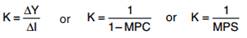
Value of investment multiplier lies b/w 1 to infinitive.
Excess demand refers to a situation when aggregate demand exceeds aggregate supply corresponding to full employment.
Inflationary gap is the gap by which actual aggregate demand exceeds the level of aggregate demand required to establish full employment.
It measures the extent of excess demand.
Deficient Demand: When AD falls short of AS at full employment it is called deficient demand. In other words, AD < AS at the level of full employment. It is called deficient demand.
Deflationary gap is the gap by which actual aggregate demand is less than the level of aggregate demand required to establish full employment.
It measures the extent of deficient demand.
Methods to control excess demand or deficient demand:
1. Fiscal Measures or Fiscal Policy
a. Change in Tax
b. Change in Public expenditure
c. Change in Public borrowing
d. Deficit financing (Printing new notes)
2. Monetary Measures or Monetary Policy
a. Quantitative measures
i. Bank rate
ii. Cash Reserve Ratio
iii. Statutory Liquidity Ratio
iv. Open Market operation
b. Qualitative/Selective measures
i. Marginal requirement
ii. Rationing of credit
iii. Direct Action
iv. Moral Suasion